This section defines some useful functions of signals (vectors).
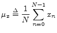
The mean of a
signal ![]() (more precisely the ``sample mean'') is defined as the
average value of its samples:5.5
(more precisely the ``sample mean'') is defined as the
average value of its samples:5.5
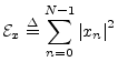
The total energy
of a signal ![]() is defined as the sum of squared moduli:
is defined as the sum of squared moduli:
In physics, energy (the ``ability to do work'') and work are in units
of ``force times distance,'' ``mass times velocity squared,'' or other
equivalent combinations of units.5.6 In digital signal processing, physical units are routinely
discarded, and signals are renormalized whenever convenient.
Therefore,
![]() is defined above without regard for constant
scale factors such as ``wave impedance'' or the sampling interval
is defined above without regard for constant
scale factors such as ``wave impedance'' or the sampling interval ![]() .
.
The average power of a signal ![]() is defined as the energy
per sample:
is defined as the energy
per sample:
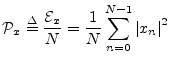
Power is always in physical units of energy per unit time. It therefore makes sense to define the average signal power as the total signal energy divided by its length. We normally work with signals which are functions of time. However, if the signal happens instead to be a function of distance (e.g., samples of displacement along a vibrating string), then the ``power'' as defined here still has the interpretation of a spatial energy density. Power, in contrast, is a temporal energy density.
The root mean square (RMS) level of a signal ![]() is simply
is simply
![]() . However, note that in practice (especially in audio
work) an RMS level is typically computed after subtracting out any
nonzero mean value. Here, we call that the variance.
. However, note that in practice (especially in audio
work) an RMS level is typically computed after subtracting out any
nonzero mean value. Here, we call that the variance.
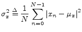
The variance (more precisely the sample variance) of the
signal ![]() is defined as the power of the signal with its mean
removed:5.7
is defined as the power of the signal with its mean
removed:5.7
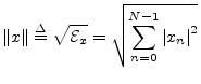
The norm (more specifically, the ![]() norm, or
Euclidean norm) of a signal
norm, or
Euclidean norm) of a signal ![]() is defined as the square root
of its total energy:
is defined as the square root
of its total energy: