If you're the sort of person who is thinking that all the algebraic
analysis was just great to read about, but so confusing, fear not.
There is indeed quite a lot to understand in all of those equations
above. For example, examining our basic parallel rate equation
(4.9), we see that if ![]() it will ALWAYS prevent us
from profitably reaching
it will ALWAYS prevent us
from profitably reaching ![]() for a fixed amount of work.
for a fixed amount of work.
What, you say? You can't see that even if ![]() goes to zero,
the
goes to zero,
the ![]() diverges, and for some value of
diverges, and for some value of ![]() (which we could
easily find from calculus, if we hadn't taken a sacred oath not to put
any calculus in this discussion) the overall rate begins to degrade?
(which we could
easily find from calculus, if we hadn't taken a sacred oath not to put
any calculus in this discussion) the overall rate begins to degrade?
Well, then. Let's Look at it. A figure is often worth a thousand
equations. A figure can launch a thousand equations. A figure in time
saves nine equations. Grown fat on a diet of equations, gotta watch my
figure. We'll therefore examine below a whole lot of figures generated
from equation (4.9) for various values of ![]() ,
, ![]() , and so
forth.
, and so
forth.
Let's begin to get a feel for real-world speedup by plotting
(4.9) for various relative values of the times. I say relative
because everything is effectively scaled to fractions when one divides
by ![]() as shown above. As we'll see, the critical gain
parameter for parallel work is
as shown above. As we'll see, the critical gain
parameter for parallel work is ![]() . When
. When ![]() is large (compared to
everything else), life could be good. When
is large (compared to
everything else), life could be good. When ![]() is not so large,
in many cases we needn't bother building a beowulf at all as it just
won't be worth it.
is not so large,
in many cases we needn't bother building a beowulf at all as it just
won't be worth it.
In all the figures below, ![]() (which sets our basic scale, if you
like) and
(which sets our basic scale, if you
like) and
![]() . In the first three figures
we just vary
. In the first three figures
we just vary
![]() for
for ![]() (fixed). Note that
(fixed). Note that
![]() is rather boring as it just adds to
is rather boring as it just adds to ![]() , but it can be
important in marginal cases.
, but it can be
important in marginal cases.
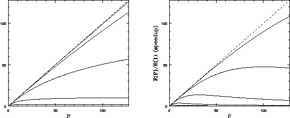
![]() (the first figure) is the kind of scaling one sees when
communication times are negligible compared to computation. This set of
curves (with increasing
(the first figure) is the kind of scaling one sees when
communication times are negligible compared to computation. This set of
curves (with increasing ![]() ascending on the figure) is roughly what
one expects from Amdahl's Law, which was derived with no consideration
of IPC overhead. Note that the dashed line in all figures is perfectly
linear speedup. More processors, more speed. Note also that we never
get this over the entire range of
ascending on the figure) is roughly what
one expects from Amdahl's Law, which was derived with no consideration
of IPC overhead. Note that the dashed line in all figures is perfectly
linear speedup. More processors, more speed. Note also that we never
get this over the entire range of ![]() , but we can often come close for
small
, but we can often come close for
small ![]() .
.
![]() is a fairly typical curve for a ``real'' beowulf. In it
one can see the competing effects of cranking up the parallel fraction
(
is a fairly typical curve for a ``real'' beowulf. In it
one can see the competing effects of cranking up the parallel fraction
(![]() relative to
relative to ![]() ) and can also see how even a relatively small
serial communications overhead causes the gain curves to peak well short
of the saturation predicted by Amdahl's Law in the first figure. Adding
processors past this point costs one speedup. In many cases this
can occur for quite small
) and can also see how even a relatively small
serial communications overhead causes the gain curves to peak well short
of the saturation predicted by Amdahl's Law in the first figure. Adding
processors past this point costs one speedup. In many cases this
can occur for quite small ![]() . For many problems there is no
point in trying to get hundreds of processors, as one will never be
able to use them.
. For many problems there is no
point in trying to get hundreds of processors, as one will never be
able to use them.
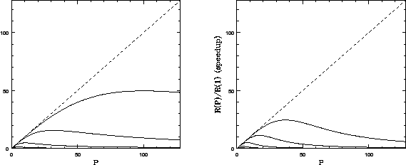
![]() (the third figure) is more of the same. Even with
(the third figure) is more of the same. Even with
![]() , the relatively large
, the relatively large ![]() causes the gain to peak
well before 128 processors.
causes the gain to peak
well before 128 processors.
Finally, the last figure is ![]() , but this time with a quadratic dependence
, but this time with a quadratic dependence ![]() . This might result if the
communications required between processors is long range and constrained
in some way, as our ``all nodes communicate every step'' example above
showed. There are other ways to get nonlinear dependences of the
additional serial time on
. This might result if the
communications required between processors is long range and constrained
in some way, as our ``all nodes communicate every step'' example above
showed. There are other ways to get nonlinear dependences of the
additional serial time on ![]() , and they can have a profound effect on
the per-processor scaling of the speedup.
, and they can have a profound effect on
the per-processor scaling of the speedup.
What to get from these figures? Relatively big ![]() is goooood.
is goooood.
![]() is baaaad. High powers of
is baaaad. High powers of ![]() multiplying things like
multiplying things like
![]() or
or ![]() are baaaaad. ``Real world'' speedup curves
typically have a peak and there is no point in designing and
purchasing a beowulf with a hundred nodes if your calculation reaches that scaling peak at ten nodes (and actually runs much, much
slower on a hundred). Simple stuff, really.
are baaaaad. ``Real world'' speedup curves
typically have a peak and there is no point in designing and
purchasing a beowulf with a hundred nodes if your calculation reaches that scaling peak at ten nodes (and actually runs much, much
slower on a hundred). Simple stuff, really.
With these figures under your belt, you are now ready to start
estimating performance given various design decisions. To summarize
what we've learned, to get benefit from any beowulf or cluster
design we require a priori that ![]() . If this isn't true
we are probably wasting our time. If
. If this isn't true
we are probably wasting our time. If ![]() is much bigger than
is much bigger than
![]() (as often can be arranged in a real calculation) we are in luck,
but not out of the woods. Next we have to consider
(as often can be arranged in a real calculation) we are in luck,
but not out of the woods. Next we have to consider ![]() and/or
and/or
![]() and the power law(s) satisfied by the additional
and the power law(s) satisfied by the additional ![]() -dependent
serial overhead for our algorithm, as a function of problem size. If
there are problem sizes where these communications times are small
compared to
-dependent
serial overhead for our algorithm, as a function of problem size. If
there are problem sizes where these communications times are small
compared to ![]() , we can likely get good success from a beowulf or
cluster design in these ranges of
, we can likely get good success from a beowulf or
cluster design in these ranges of ![]() .
.
The point to emphasize is that these parameters are at least partially
under your control. In many cases you can change the ratio of ![]() to
to
![]() by making the problem bigger. You can change
by making the problem bigger. You can change ![]() by using a
faster communications medium. You can change the power scaling of
by using a
faster communications medium. You can change the power scaling of ![]() in the communications time by changing the topology, using a switch, or
sometimes just by rewriting the code to use a ``smarter'' algorithm.
These are some the parameters we're going to juggle in beowulf design.
in the communications time by changing the topology, using a switch, or
sometimes just by rewriting the code to use a ``smarter'' algorithm.
These are some the parameters we're going to juggle in beowulf design.
There are, however, additional parameters that we have to learn about. These parameters may or may not have nice, simple scaling laws associated with them. Many of them are extremely nonlinear or even discrete in their effect on your code. Truthfully, a lot of them affect even serial code in much the same way that they affect parallel code, but a parallel environment has the potential to amplify their effect and degrade performance far faster than one expects from the scaling curves above. These are the parameters associated with bottlenecks and barriers.