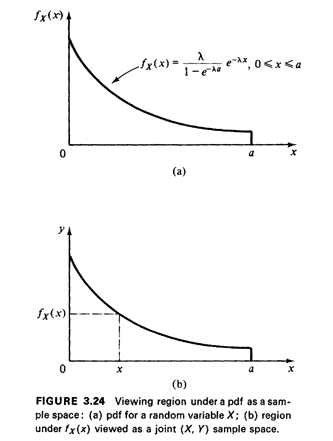


3.4.1 A Geometrical Probability Interpretation of PDF'sSomewhat surprisingly, the assumption of spatially uniform and independent points appears in virtually every probability density function that we confront. We can understand this by considering an arbitrary random variable X with pdf fx(x), - < x < + < x < +  (Figure 3.24a). Instead of
viewing the "area under the curve" fx(x) as representing
probability, we can view that region as a joint sample space for
random variables (X, Y) that are uniformly
distributed over the sample space (Figure 3.24b). Random variable
X, as before, assumes experimental values - (Figure 3.24a). Instead of
viewing the "area under the curve" fx(x) as representing
probability, we can view that region as a joint sample space for
random variables (X, Y) that are uniformly
distributed over the sample space (Figure 3.24b). Random variable
X, as before, assumes experimental values -
 <
x < + <
x < + , and for random variable Y we have 0 , and for random variable Y we have 0
 y y  + + . Since
the area under the curve fx(x) is 1, the joint pdf
fx,y(x, y) has height equal to I over the sample space. Given
any particular value of X, say X = x, we have 0 . Since
the area under the curve fx(x) is 1, the joint pdf
fx,y(x, y) has height equal to I over the sample space. Given
any particular value of X, say X = x, we have 0  {Y
| X = x} {Y
| X = x} fx(x); in this case {Y| X = x) is uniformly
distributed over (0, fx(x)]. This must be an acceptable
interpretation since, as before, fx(x); in this case {Y| X = x) is uniformly
distributed over (0, fx(x)]. This must be an acceptable
interpretation since, as before,

Now successive independent experiments that yield values for the random variable X can be viewed as successive independent experiments in which 
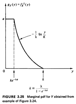
(X,Y) are uniformly distributed over this (X, Y) sample space, and in which we are only interested in the experimental value of X. This "geometrical probability" interpretation for fx(x) will be of value in our work. Suppose thatfx(x) is strictly monotonically decreasing with x. Then there exists an inverse function gy(y) = fx-1 (y) which can be viewed as the pdf for the random variable Y. The monotonicity assumption is true for the example of Figure 3.24, and a simple logarithmic transformation shows that 
for  . This function, which is simply fx(x)
"flipped on its side and turned around" is shown in Figure
3.25. [Note that no scaling is required . This function, which is simply fx(x)
"flipped on its side and turned around" is shown in Figure
3.25. [Note that no scaling is required

since, as mentioned before, the "area of the sample space" in this case must be one because 
The same reasoning can be applied in reverse. That is, we may, in
fact, have a spatial situation involving uniformly
independently distributed points over some region and we may
require the probability laws of the random variables
X and Y. Since few geographical regions have area specified to
equal unity, care must be taken to scale appropriately the
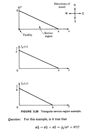
marginal pdf's for X and Y so that they integrate to 1. Utilizing the "geometrical probability" interpretation for pdf's,
by inspection we obtain the marginal pdf's for X and Y,
both triangular, as shown in Figure 3.26. From earlier work the
mean travel distance is found to be
E[D] = E[X + Y] = E[X] + E[ Y] = 1/3(a + b) (3.59)

Why or why not? Further work: See Section 3.7.3 and Problems 3.30 and 3.31. |


