Suppose that we have entities distributed around the city in a completely random manner.
These entities could be employees of a particular service system, recipients of a certain
social service, emergency response units, crimes, and so on. We require a way of
describing probabilistically the numbers of entities in given subareas and spatial
interrelationships among entities. To do this, we generalize the idea of a Poisson process
in time to a Poisson process in space. We recall from Chapter 2 that for a homogeneous
Poisson process in time, the probability that exactly k Poisson events occur in a fixed
time interval [0, t] is
where  is a positive
constant interpreted as the average rate at which events are happening per unit time. The
process is called "homogeneous," because does not vary with time. is a positive
constant interpreted as the average rate at which events are happening per unit time. The
process is called "homogeneous," because does not vary with time.
Applying the same ideas in a spatial setting, first consider a homogeneous highway
segment of length l miles. From past accident records we may know that each year an
average of highway accidents occur
per mile on this type of highway. Then the number of highway accidents that occur in the
segment of length l miles can be modeled as a Poisson random variable with mean l, Here the parameter distance (l)
plays a role directly analogous to time (t). For the Poisson model to be a
reasonable one, the locations of accidents must occur consistent with Poisson- type
assumptions: (1) only nonnegative integer numbers of accidents can occur in any length of
highway; (2) the probability distribution of the number of accidents depends only on the
length of highway considered, and as this length goes to zero so does the probability of
an accident occurring there; (3) the numbers of accidents occurring in nonoverlapping
segments of highway are mutually independent random variables; and (4) given that an
accident occurs at a particular location, the chance of a second accident occurring at the
identically same location is zero. Assumptions (1) and (3) appear fairly reasonable for
most highways. Since different parts of a highway (e.g., curves versus straight-aways) can
be associated with different risks of accident, the first part of assumption (2) may have
to be modified in practice to allow for a spatially varying (nonhomogeneous)
Poisson process, with accompanying (x)
defined so that (x)dx = probability of
an accident occurring (during a year) in the road interval x to x + dx. A highway with
overpasses, bridges, and other discernible high-risk points may yield a positive
probability of at least one accident during a year at these points (e.g., at the base of
an overpass), thereby negating the second part of assumption (2). Such high-risk points
would also tend to negate assumption (4), which also might be invalidated by
chain-reaction multiple-car accidents (such as those that occasionally occur in fog) if
those are counted in accident data as more than one accident.
In practice, almost any real system will demonstrate a nonperfect degree of conformity
with the postulates of the Poisson process. In assessing the applicability of the Poisson
model, the modeler must weigh the benefits of applying the Poisson model (together with
the insights it provides) against the cost of inaccuracies introduced by such a simple
model and the cost of constructing a more complex model. Sometimes a forced degree of
ignorance involving details of a system (e.g., the locations of overpasses) will
facilitate application of the model.
The ideas illustrated above for a Poisson process on a line (a highway) extend directly
to the plane (to describe entities distributed over two dimensions). Let the parameter S
denote a bounded region of the plane (or higher- dimensional space, for that matter). Let
X(S) be the number of entities contained in S. Then X(S) is a homogeneous spatial Poisson
process if it obeys the Poisson postulates, yielding a probability distribution
In this case is a
positive constant called the intensity parameter of the process and A(S) represents
the area or volume of S, depending on whether S is a region in the plane or
higher-dimensional space.
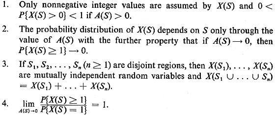
The underlying mathematical postulates of the model follow directly those of the time
Poisson process:
Generalization: As with the time Poisson process, it is not difficult to extend
these ideas to a spatially varying (nonhomogeneous) Poisson process. For instance, in the
plane if
(x, y)dxdy = P{a Poisson entity is
located in the interval x to x + dx, y to y + dy}
then in (3.96), A(S) is replaced by
In this case postulate (2) is changed to read: "The probability
distribution of X(S) depends on S only through the value of (S) with the further property that as (S)  0, then
P{X(S) 0, then
P{X(S)  1} 0." 1} 0."
|