4.7 Spatially Distributed Queues And The M/G/1 Queueing System

As we have already mentioned at the beginning of this chapter, many queueing systems in the urban environment do not fit neatly into the classical mold of a physically stationary server where prospective "customers" arrive and queue up until they receive service. For most of the emergency urban services-where "arrivals of customers" are perceived through telephone calls (or other means of telecommunication) from various locations in a citythe only place at which a "queue" can be identified is on the emergency system's dispatcher's desk (or in a computer's memory), where records indicate the time, origin, and nature of a succession of requests for service. The server, then, be it a person or a vehicle, must travel to the location of these incidents to provide the required service. In such cases we have a spatially distributed queue.
    In this section we shall discuss the simplest possible type of spatially distributed queue in which a single server has sole responsibility for a given district. This discussion will also motivate our derivation of some important results for M/G/1 queueing systems.

Example 1: Ambulance Service to an Emergency Medical Facility

Consider the case pictured in Figure 4.10: an emergency medical facility (EMF) is located at the center (the point where the diagonals intersect) of a rectangular district with dimensions X₀ � Y₀ miles. The EMF has a single ambulance vehicle associated with it, which is dispatched to emergency patients and transports them to the EMF. The ambulance, when idle, is always located at the EMF.

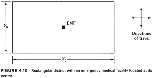
    Directions of travel are parallel to the boundaries of the district and the effective travel speeds are v_x. and v_y (constants) in the x and y directions, as shown in Figure 4.10.
    In this district, incidents (each corresponding to one emergency patient) occur as a Poisson process in time at a rate of A per hour. Incident locations are independent of each other and are uniformly distributed over the rectangular area. Every time an incident occurs, the ambulance, if at the EMF, is immediately dispatched to the location of the call, picks up the patient, and returns to the EMF. If the ambulance is away, calls queue up and are processed in a FIFO order. We shall assume for now that no calls are ever lost, no matter how long they have to wait. We shall also assume that the pdf for the time, Z, that the ambulance spends at the location of each call for service is known and is given by f_z(z) with an expectation Z and a variance _z.
    The service time, S, in this system clearly consists of a   "travel-time" component and a "time on the scene" component. Assuming that effective travel speeds are identical on both the EMF-to-incident and the incident-toEMF portions of each trip, we have

where T_x = D_x/v_x, and T_y = D_y/v_y, and D_x and D_y are defined as the distances along the x and the y axes, respectively, from (to) the EMF to (from) the location of an incident.
    With the techniques presented in Chapter 3, it is an easy matter to obtain the expected value of S, which for consistency with our queueing theory notation we shall denote as 1/:

    If f_z(z), as we have already assumed, is known, it is also possible, at least in principle, to obtain an expression for f_s(s), the service-time pdf. The derivation, however, even for the simple situation described here, promises to be tedious and time-consuming and will be omitted. It suffices to note that f_s(s) cannot be a negative exponential pdf [unless f_z(z) is negative exponential and the expected time on the scene is much larger than the average round-trip time, in which case it can be argued that 1/ Z and, therefore, that f_s(s) is approximately negative exponential as well ⁷]. It is therefore clear that results derived for the single-server queueing systems we have seen so far (M/M/1) do not apply in this case, since the service-time distribution at hand is a "general" one.

We shall now proceed to derive several important results for this M/G/1 queueing system. Interestingly, as we shall see, most of the results require no knowledge of the service-time distribution, f_s(s), other than its mean, 1/, and variance .

    Recall first that the current state of M/M/1 (or M/M/m) queueing systems is fully described by a single item of information, the number of users (i.e., of calls in our EMF example) currently in the system. Knowledge of this number is sufficient to describe all the past history of the queueing system, as far as the future is concerned. For instance, if it is known that at some time instant, t, there are exactly n (> 0) calls in a M/M/1 system (with one call receiving service and the other n - 1 calls in the waiting line), then we can immediately state that the probability thatin the next t a service will be completed is equal to t-independently of what else has happened in the past at that M/M/1 system. For M/G/1 systems, however, this probability also depends on how long ago service began to the call that is currently receiving service. Thus, a complete description of the current state of a M/G/1 system requires, in general, specification of the values of two random variables, the number of calls currently in the system, and the time since the current service began, the latter of which is a continuous random variable. These complications make the mathematical analysis of M/G/1 systems more difficult than that of M/M/1 or M/M/m systems.
    Of the several different approaches that have been developed, the simplest one uses the trick of focusing attention on certain specific instants in time, known as epochs, when knowledge of only the number of calls currently in the queueing system is sufficient to specify its current state. Those instants of time are the times of completion of a service by the server (i.e., the instants after the ambulance has returned to the EMF and delivered a patient, in the case of our example).
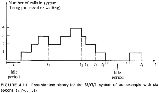
    Let us then indicate these time instants as t₁, t₂, t₃ . . . with ti, representing the instant when service to the ith patient to be transported to the EMF (beginning with some arbitrary time t = 0) is completed. A specific example for a hypothetical M/G/1 queueing system is shown in Figure 4.11.

We can then define:

N = number of calls in the queueing system (i.e., the number of patients/incidents waiting for service) just after the instant t_i-1 when service to the (i - 1)th patient is completed

R = number of new calls that arrive at the queueing system during the service time of the next patient to receive service (patient i)

N' = number of calls in the queueing system just after t_i, the instant of completion of service to patient i

    Note that, by definition, R includes only those calls that arrive at the queueing system after service to the next patient (patient i) has started. This is important for the cases when, upon completion of a service, the queueing system is left empty (i.e., no more calls left to serve). For instance, the value of R for the time interval between t₅ and t₆, is 0 (not 1) for the sample case shown in Figure 4.11.
    The following relationship exists between the random variables N, R, and N':

The probability _r, that exactly r calls arrive during a service time is given by

r = P{number of new arrivals during a service time= r} = p_R(r)

where, as above, f_s(s) represents the pdf for the service time. For any given pdf f,(s), it is then possible to determine the probabilities _r.

Exercise 4.5 How is (4.63) justified?

Hint: Given that a service lasted exactly a time t, what is the  probability that r new calls arrived during that service time?

For r = 0, 1, 2,. . . , we have

So (4.64) and (4.65) give the state-transition probabilities for successive epochs for the M/G/1 system. The state-transition diagram for our M/G/1 system, at the epochs is now shown in Figure 4.12. A state is defined by

"the number of calls present at the time when a service is completed." Note that the state-transition diagram of Figure 4.12 is no longer of the birth-and-death type.
    In the analysis that follows, we shall be interested only in the expected values , , , and _q, which can be derived without using the state-transition diagram. We shall, therefore, ignore Figure 4.12 from here on.
    Let us define a random variable such that

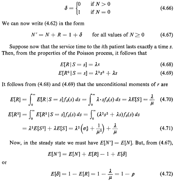
Note that (4.72) has a very real meaning: from the definition of  , it follows that E[] is equal to the fraction of epochs, ti at which the queueing system will be found empty upon completion of a service. It follows that (4.72) cannot be meaningful unless ⁸
< 1 (< ). This is also the condition under which steady state exists for M/G/1 systems.

  Let us now square both sides of (4.67) to obtain

where we have used the facts that = and that 2N = 0 (both  resulting directly from the definition of ). Taking now the expected values of both sides of (4.73) and noting that  in the steady state E[(N')^2]1 = E[N^2], we have

We have used the asterisk in (4.74) to indicate that * denotes the expected number of users in the system at the instants that follow the service completions on which we have concentrated, the epochs.
    It turns out that * is equal to , the expected number of calls in the queueing system that would be observed by someone arriving at a random time with the system in the steady state. To show this, it suffices to show that the steady-state pmf for the number in the system at the instants of service completion is identical to the steady-state pmf for the number in the system at any random instant. This we now proceed to do in a rather informal way. We define

_n = steady-state probability that just after the completion of a service there are n calls left in the queueing system

P_n  = steady-state probability that a call arriving at the system at a random time will find n calls in the queueing system

J_n = number of "downward jumps" from n + 1 to n (in the number of  calls in the queueing system) which are observed during a time interval T

J = J_n = total number of downward jumps in the number of calls in the queueing system observed during the time interval T

K_n = number of "upward jumps" from n to n + 1 (in the number of calls in the queueing system) which are observed during the time interval T

K = K_n = total number of upward jumps in the number of calls in the queueing system observed during the time interval T

    Obviously, downward jumps are due to service completions and upward jumps are due to call arrivals. Obviously, too, the quantities J_n and K_n can differ by at most 1 unit during any time interval T.
    Assuming that the queueing system does reach steady state, we have, from the definition of  _n, that

Also, since steady state is reached, the number of upward jumps must be about the same as the number of downward jumps (i.e., the ratio of J to K must go to 1 as T goes to infinity). From this, plus the fact that J_n and K_n differ at most by one and from (4.75), we then have

    The right-hand side above is the steady-state probability that the system is in state n at the instant of an arrival. Arrivals, however, occur in a Poisson manner, meaning that the  instants of arrivals are completely random! Thus, lim _t   (K_n/K) = P_n and we have shown that

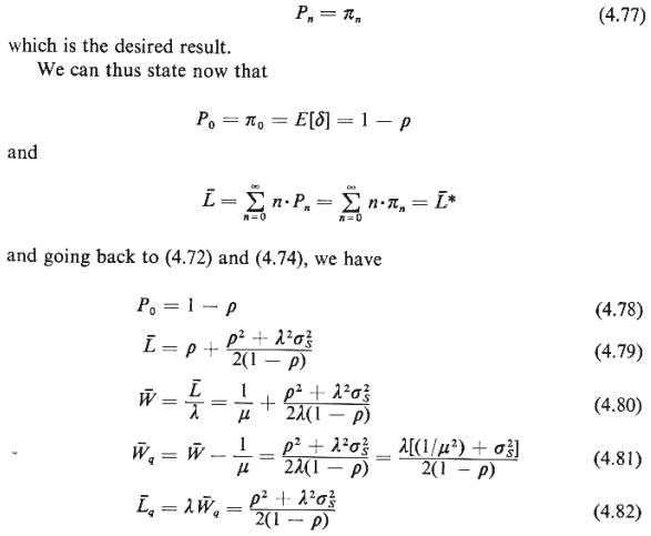
for the M/G/1 queueing system. These results are valid for steady-state conditions which exist whenever

    Expressions (4.78)-(4.82) are remarkable for their simplicity, since they apply to any service-time distribution. [In fact, in deriving these expressions we made no assumptions whatsoever about the specific form of f_s(s).] They are usually referred to as the "Pollaczek-Khintchine formulas." To use them, all that is needed to know about the service time is its expected value and its variance-which is certainly most convenient in practical applications. It is also important to note that (as well as , _q, and _q) depends on the variance of the service times: increasing the consistency of service (i.e., reducing the variance of service times) improves the performance  of the service facility.
    Several additional results have been obtained with regard to the   M/G/1 queueing system. For instance, from (4.78) we can conclude that the following ratio holds:

E[length of busy period] = fraction of time system is busy = /(1- )
  E[length of idle period] = fraction of time system is idle

But since E[Iength of idle period] = 1/ (since we have Poisson arrivals with rate ), it can be concluded that

Interestingly, (4.83) is identical with (4.43), the expression for the expected length of the busy period for M/M/1 queueing systems.
    For a given service time pdf, f_s(s), it is also possible to obtain expressions (or numerical estimates) for the steady-state probabilities, P_n. This is accomplished by first obtaining an expression for the geometric transform of these probabilities (see, for instance, [GROS 74]).

Example 1 (continued)

To illustrate some of the above, let us take X_O = 2 miles, Y_O = 1 mile, v_x, 30 miles/hr, v_y, = 20 miles/hr, = 10 minutes, and = 25 minutes².

Solution

It follows from (4.60) and (4.61) that l/ = 13.5 minutes and = 27.1 minutes. Thus, the service rate = 4.44 calls/hr. We can then derive the following table, for different demand (call) rates, , under steady-state conditions:

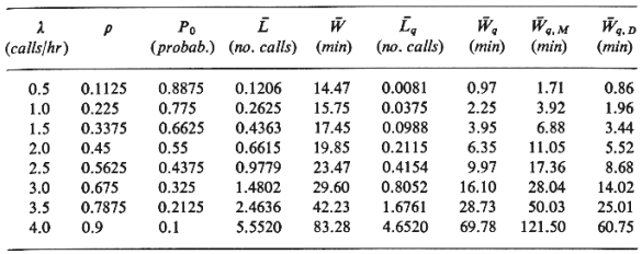
    The quantities P_O, , ,_q , and _q in this table have been computed by using relations (4.78)-(4.82). _{q,M and q.D, the quantities listed in the two rightmost columns represent  the average waiting time for the corresponding M/M/1 and M/D/1 systems, respectively. That is, q,M has been computed for  a single-server system with negative exponential service time distribution and an expected service time, 1/, of 13.5 minutes; similarly, q,D corresponds to a constant service time equal W 13.5 minutes. Since an M/M/1 system can be viewed as just a special case of M/G/1, it is hardly surprising that when we set = 1/ (negative exponential service times) in (4.79)-(4.82), the expresssions for the corresponding M/M/1 quantities are obtained. (Try one!) Similarly, the expressions for the M/D/1 system can be obtained by setting = 0 in (4.79)-(4.82). A particularly simple and useful relationship to remember is that}

    As one might expect from the fact that < 1/ in our example, the values of _q, for all values of in the table fall between the corresponding values of _q,m and _q,d. In fact, there is a particularly convenient form for expressions (4.79)-(4.82) that brings out clearly the significance of the term that includes the variance of the service time: we can use the coefficient of  variation C_s,( _s / E[S] = _s. ) for the service time to rewrite, say, (4.79) as

(Remember that for negative exponential service times C_s = 1 and  for constant service times C_s = 0.)
    Finally, to conclude the exanple, we might want to review the table of numerical results to assess the Performance of the ambulance service that we have described. It is interesting, for instance, that at an arrival rate of 1.5 calls/hr, the average delay before the ambulance is dispatched to a random call for service is about 4 minute-longer than what it takes for the ambulance, on the average, to travel from the EMF to the point from which the call has originated and back (= 3.5 minutes). And this, despite the fact that, for = 1.5, the ambulance is busy (traveling or at the scene of an incident) only about one third of the time. It is thus very likely that emergency medical service administrators would find the level of service (as manifested by the average dispatch delay, _q) provided by this single ambulance emergency medical system to be unacceptable for  call rates greater than 1.5 or, at most, 2.0 calls/hr.
    What to do, then? We might attempt to speed up service (reduce 1/) or "standardize" the service (reduce ²_s). Suppose that a 20 percent decrease could be achieved for 1/  [i.e., we could achieve 1/' = (13.5)(0.8) = 10.8 minutes]. Then for, say, = 3.0, we would obtain _q' = 7.82 (assuming that stays constant at 27. 1). This is a better than 50 percent reduction in average S dispatch delay!
    Suppose, instead, that we could reduce the standard deviation of service times by 20 percent [i.e., that we could achieve ''_s = (0.8)(27.1)^1/2 or, in other words ()" =  (0.64)(27.1) = 17.341. Then for = 3.0, and assuming that 11p remains constant at 13.5, we would obtain _q'' = 15.35 minutes or an improvement of only about 5 percent over the original _q of 16.1 minutes. In general, reductions in expected service times are usually much more effective than comparable reductions in the variance of service times. This should be obvious from the fact that changes in the expected service time, 1/ affect both the numerator and denominator of (4.79)-(4.82) by changing the utilization factor, p.
    When it is not possible to reduce 1/ or to achieve improved perfor S mance for a given demand rate , one has to resort to more drastic measures, such as increasing the number of ambulances in our present example or reducing the area of responsibility of the EMF (and thus as well). With m ambulances at hand (m > 1) that would mean an M/G/m queueing system, which we proceed to discuss next. A more "complicated" spatially distributed M/G/1 queueing system will be discussed in Section 5.2.