


5.4.3 Three-Server Example (infinite Line Capacity)To serve as both an example of the use of the hypercube model and a
vehicle to derive its general mathematical structure, we consider the
simple three-server city shown in Figure 5.11. This city is partitioned
into 10 geographical atoms, each acting as an independent Poisson
generator of service requests. For ease of presentation, we will assume
that the mean service time of each unit n is the same known
constant 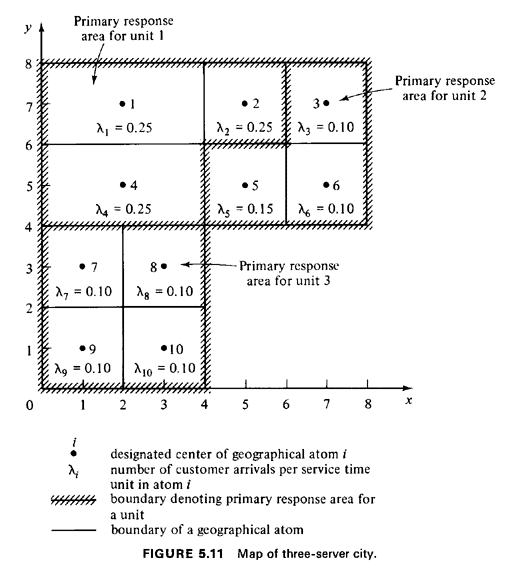
Throughout the remainder of this chapter, we assume that the hypercube model has infinite queue capacity. Some results for the zero-capacity case are presented in the problems at the end of the chapter. The rates 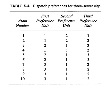
If we are only interested in workload-oriented performance measures,
it is not necessary to specify the interatom travel-time matrix
In this example we have set all the mean service times equal to the
same constant. With this restriction, the queueing system in the
aggregate (if one is not concerned with the identity of busy servers) is
simply the M / M / N system, as discussed in Chapter 4. But the
state space in which the identities of servers are retained is more
complicated than the set of nonnegative integers which is adequate for
the M / M / N model. Symbolically, if we say that
bn = state of server n (bn =
0 for "free," or bn = 1 for "busy"), the system state
is given by B =
{bN,bN-1 ,...,
b1}The collection of all possible B's is
denoted by CN, corresponding to the vertices of an
N-dimensional hypercube. The weight of B, denoted
w(B), is equal to the number of busy servers in the state
B; thus, w(B) = For the case of equal mean service times, we can use the concept of weight of a state to relate the hypercube state space to the simpler M / M / N state space. This equivalence is obtained by collecting together all states having equal weight, say w0; their summed probability of occurrence is equal to the comparable probability of state Sw0, occurring in the M / M / N model (using the results of Chapter 4). For instance, the states 001, 010, and 100 all have weight 1, and their summed probability must equal the probability of state S1, in the M / M / N model. One way of demonstrating this equivalence is shown in Figure 5.12, in which all hypercube states having equal weight are grouped together vertically. Figure 5.12 also shows explicitly the infinite tail that augments the hypercube state space to allow the possibility of a queue. Since this infinite tail behaves in just the same manner as the infinite tail of the M / M / N model, we will not explicitly add it to the more geometrically oriented "cubic" state space shown in Figure 5.13. In this figure, the collection of states 001, 010, and 100 can be seen to intersect a plane at a generalized 45o angle to the origin; that is, each side of the cube cut by this plane is cut at a 45o angle and, measured along the cube's edges, the plane is a distance 1 from the origin. We can generalize this concept to N dimensions, defining Hn Here Hn is the set of states intersecting a hyperplane located a distance n from the origin (distance measured in a "right-angle" way along edges of the cube), situated at a generalized 45o angle with respect to the origin. We sometimes refer to Hn as the nth hyperplane from the origin, recognizing that, in fact, it is made up of only a finite number of points (states). Exercise 5.1: Argue that the number of points or states in Hn is equal to In extending the model to N dimensions it becomes cumbersome to denote each state as an N-digit binary number. Thus, we are motivated to use a state indexing scheme that corresponds in a natural way to the binary state representation. The index we choose is simply the decimal integer numerical value associated with each binary representation. For example, for the N = 3 unit problem, we have 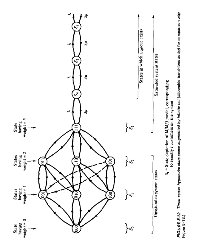
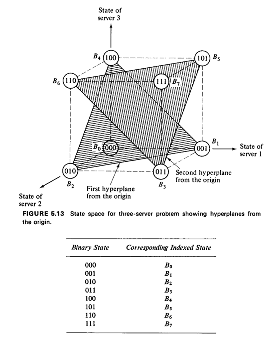 This correspondence is shown in Figure 5.13. In general, for an N-unit problem, the indexed states run from B0 to B2N -1. For a generic state B = {bN, bN-1, . . . , b1}, its index value is simply
In the reverse direction, for each positive integer k there
corresponds a unique Bk such that State-to-state transitions. With the hypercube model transitions occur between states just as they do with other queuing models. The hypercube model assumes that only one unit is assigned to each service request. Thus, assuming that it is virtually impossible for two requests to arrive simultaneously, a transition from state (0, 0, 0) to state (0, 1, 0) would be allowable, whereas a two-step transition from state (0, 0, 0) to state (0, 1, 1) would not (since it implies that two free units become busy at the same instant). Likewise, if we assume that each of the busy units is working independently at its particular location to complete service on its current service request, it is virtually impossible for two busy units to become free simultaneously. Thus, a transition from state (1, 0, 1) to state (0, 0, 1) is allowable, whereas a two-step transition from state (1, 0, 1) to state (0, 0, 0) is not. Summarizing, any one-step transition is allowable; all multistep transitions are not allowable. Transitions can be thought of as occurring only between states in adjacent hyperplanes from the origin. One's intuition is again assisted by visualizing these transitions to occur on the hypercube. Since a one-step transition causes only one of the "O's" or "1's" to change in the system-state description (meaning that only one unit's state changes), we can visualize the transition as occurring along an edge of the hypercube. (An edge is a straight line connecting two adjacent vertices of the hypercube.) For instance, referring again to Figure 5.13, a transition from state (0, 0, 1) to state (1, 0, 1) occurs along the rightmost edge of the cube. As an example of combining the concepts of state and transition, consider our three-unit city, which starts with all units free. Suppose that the following events then occur:
Recalling that atom 6 is within unit 2's primary response area, the request for service from atom 6 would result in unit 2 becoming busy, yielding a transition from state (0, 0, 0) to state (0, 1, 0). Likewise, the next request for service would cause unit 1 to become busy, resulting in a transition from state (0, 1, 0) to state (0, 1, 1). Next, when unit 2 becomes free, the system makes a transition to state (0, 0, 1). Next, when a request for service arrives from atom 4, in unit 1's primary response area, we note that unit 1 is already busy servicing a request. Since the primary backup unit, unit 3, is available, it is dispatched to the scene, resulting in an interresponse area assignment. The system now undergoes a transition from state (0, 0, 1) to state (1, 0, 1). Finally, when a request arrives from atom 3, unit 2 is dispatched, causing the system to enter a saturation state (1, 1, 1). (Any additional service requests arriving while all servers are busy would be delayed in queue.) Summarizing the example above, the sequence of states occupied by the system is as follows: (0, 0, 0) (0, 1, 0) (0, 1, 1) (0, 0, 1) (1, 0, 1) (1, 1, 1) Now the value of the cube as an aid in visualizing the behavior of the system is seen in Figure 5.14, which depicts the states occupied and the state-tostate transitions as a sequence of connected trips along edges of the cube. 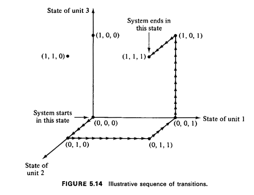
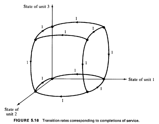
Transition rates on the hypercube. We are now ready to link the arrival rates and the service rates to states and transitions on the hypercube. Referring again to Figure 5.13, suppose that the system is in the "empty state," (0, 0, 0). Recall that 0.75 request for service arrives per unit time from unit 1's primary response area, 0.35 from unit 2's primary response area, and 0.40 from unit 3's. Also recall that time is measured in mean service time units. Then, from state (0, 0, 0), there is a rate of transition to state (0, 0, 1) equal to 0.75 request per unit time. Likewise, there is a rate of transition from state (0, 0, 0) to state (0, 1, 0) equal to 0.35 per hour and to state (1, 0, 0) equal to 0.40 per unit time. These state-to-state transition rates can be drawn onto the cube as shown in Figure 5.15. In a similar manner, the transition rate from any state to any adjacent state having one less unit busy is 1 per unit time, and these transition rates are depicted in Figure 5.16. We have now filled in the transition rates from state (0, 0, 0) and all the rates corresponding to completions of service. For convenience, the latter type of transitions are called "downward" transitions, indicating that the total number of busy units has dropped down by one. Transitions that result in a unit being dispatched are called "upward" transitions, because the total number of busy units has gone up by one. The careful reader will notice that we have not yet specified most of the upward transitions. This is due to the fact that upward transition rates depend on the dispatcher's selection strategy, and this complicates the specification of most of the upward transition rates. One further set of upward transition rates is particularly easy to
specify. Since all service requests that arrive are serviced immediately
(i.e., they incur no queue delay) if at least one response unit is
available, all states that are unit distance from the saturation state
(states 011, 101, and 110 in our example) must have an upward transition
rate equaling the total system-wide request rate 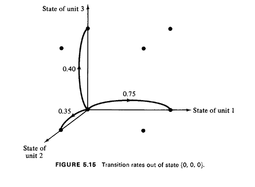
To compute the values of the remaining upward transition rates, consider for instance the transition rate from state 001 to state 101. This rate will consist of the sum of two rates: the rate of service requests from unit 3's primary response area plus the overflow rate from that part of unit 1's primary response area assigned to unit 3 as the first backup unit. The first rate is simply 0.40 request per unit time. The second is the arrival rate from atom 4 (0.25 request per unit time), since the first backup unit for atom 4 (in unit 1's primary response area) is unit 3. (Unit 2 is the first backup unit for the other atoms in unit 1's primary response area.) Thus, the net upward transition rate from state 001 to state 101 is (0.40 + 0.25) = 0.65 request per unit time. In a like manner, the remaining upward transition rates can be found. The entire state-transition diagram for this example (excluding the infinite tail) is shown in Figure 5.17. Steady-state balance equations. Although it is instructive to visualize this process on a three-dimensional cube (or a square, for N = 2), no such visual aids are available for N > 3. Thus, one should be able to write down the equilibrium equations of balance without resorting to the visual aid. We do this below, utilizing our knowledge that sums of steady-state probabilities along given hyperplanes from the origin must equal corresponding state probabilities from the simple M / M / N model. 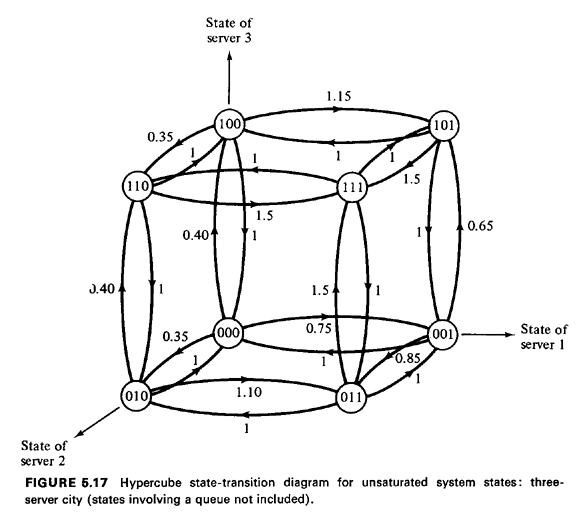
We define From the M / M / 3 model (4.44), setting  = 1.5, = 1.5,  = 1, we have = 1, we have
Using these results, we can now write the hypercube equilibrium equations for nonsaturated system states:
We solve this set of equations by eliminating the following variables, in order, by use of the designated equations: 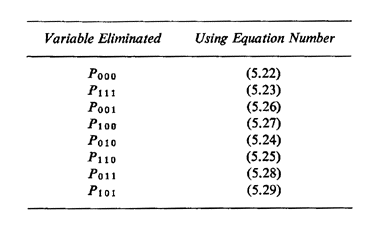
After about 15 or 20 minutes with an electronic hand calculator, we arrive at the following values for the state probabilities: P000 = 0.21053 P001 = 0.13669 P010 = 0.08863 P100 = 0.09047 P110 = 0.05301 P101 = 0.08894 P011 = 0.09489 P111 = 0.11842 |