

7.2.2 Simulating the Locations of Urban EventsWe now turn to what is perhaps the most fundamental geometrical question in the simulation of urban service systems: How do we simulate the locations of incidents, requests for service, or other events of interest which are distributed according to some prespecified probability law? Suppose that the city (or part of the city) which is to be simulated is partitioned into small-area reporting zones, such as census blocks or police reporting areas or voting districts. If each reporting zone is small enough to be considered homogeneous, it would not be unreasonable to assume that locations of events within each zone are uniformly distributed. The concept of the zone is identical to the concept of the atom (Chapter 5) or of the demand-generating node (Chapter 6). We choose to use the term "zone" here because it conveys better the idea of geographical entities of varying areas and shapes with which we are now dealing. To obtain a sample location from within the city, the following two-step procedure can be used:
The second step is by no means trivial if we allow the zones to have
arbitrary shapes-as we should to allow for maximum flexibility. An
approach that works well in this respect is the use of the rejection
method of sampling (Section 7.1) to generate sample values for two
random variables simultaneously. We assume that any given zone can be
modeled as a polygon with n sides (n arbitrary) having no special
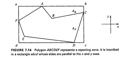
properties such as convexity.5 Suppose that we enclose that polygon in
the smallest rectangle fully containing it, with the sides of the
rectangle constrained to be parallel to some prespecified set of
coordinate axes (Figure 7.14). Then, using two random

numbers, a candidate point that has a uniform distribution over the rectangle is obtained. If this point is also within the polygon, it is accepted as the sample value; otherwise, it is rejected and new points are generated until one is accepted. The probability that any candidate point will be accepted is equal to the ratio of the area of the polygon (AP) to the area of the rectangle of accuracy, zones of any shape as polygons. (AR). The number of candidate points that have to be generated until one is accepted is a geometrically distributed random variable with mean AR/AP. For reasonably compact polygons, this number, reflecting sampling efficiency, is usually less than 2 (and often quite close to 1). How does the computer determine whether a particular candidate point in the rectangle is inside or outside the polygon of interest? An effective way to deal with this problem is the point-polygon method. Point-polygon method. The point-polygon method answers the following
question: "Given a point (x, y) and a polygon specified by the n
clockwise
ordered vertices (x1, y1), (x2,
y2), . . . , (xn, yn), is the point
(x, y) contained within the polygon?" The basic idea of the method is to
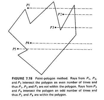
extend a ray in any direction from the point in question; if the ray
intersects the sides of the polygon an odd (even) number of times, the
point is (is not) within the polygon [NORD 62, BROW 68]. Figure 7.15
illustrates this idea. The method "works" because if the point is
outside the polygon, the ray will exit the polygon each time that it
enters it, since it must end up outside the polygon; the number of exits
equaling the number of entries implies that the total number of
intersections must be an even number. If, on the other hand, the point
is within the polygon, then the number of exits e must be one greater
than the number of entrances (e - 1), because the initial exit is not
paired with an entrance; the total number of intersections 2e - I is
clearly an odd number.

The method is completely general and does not require any special properties of the polygon. It is particularly well suited for machine implementation, since the tests for intersection are quickly performed on a computer (see also Problem 7.4). 5 This is a reasonable assumption, since we can approximate, to any desirable degree |


