Frequencies in the ``Cracks''

The DFT is defined only for frequencies $\omega_k = 2\pi k f_s/N$. If we are analyzing one or more periods of an exactly periodic signal, where the period is exactly $N$ samples (or some integer divisor of $N$), then these really are the only frequencies present in the signal, and the spectrum is actually zero everywhere but at $\omega=\omega_k$, $k\in[0,N-1]$. However, we use the DFT to analyze arbitrary signals from nature. What happens when a frequency $\omega$ is present in a signal $x$ that is not one of the DFT-sinusoid frequencies $\omega_k$?

To find out, let's project a length $N$ segment of a sinusoid at an arbitrary frequency $\omega_x$ onto the $k$th DFT sinusoid:

$$\begin{eqnarray*} x(n) &\isdef & e^{j\omega_x n T} \\ s_k(n) &\isdef & e^{j\ome... ...}{\left<s_k,s_k\right>}s_k \;\isdef \; \frac{X(\omega_k)}{N}s_k \end{eqnarray*}$$

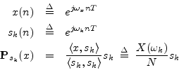
The coefficient of projection is proportional to

$$\begin{eqnarray*} X(\omega_k) & \isdef & \left<x,s_k\right> \;\isdef \; \sum_{n=... ...ac{\sin[(\omega_x-\omega_k)NT/2]}{\sin[(\omega_x-\omega_k)T/2]}, \end{eqnarray*}$$

using the closed-form expression for a geometric series sum once again. As shown in §6.3-§6.4 above, the sum is $N$ if $\omega_k=\omega_x$ and zero at $\omega_l$, for $l\neq k$. However, the sum is nonzero at all other frequencies $\omega_x$.

Since we are only looking at $N$ samples, any sinusoidal segment can be projected onto the $N$ DFT sinusoids and be reconstructed exactly by a linear combination of them. Another way to say this is that the DFT sinusoids form a basis for ${\bf C}^N$, so that any length $N$ signal whatsoever can be expressed as linear combination of them. Therefore, when analyzing segments of recorded signals, we must interpret what we see accordingly.

The typical way to think about this in practice is to consider the DFT operation as a digital filter for each $k$, whose input is $x$ and whose output is $X(\omega_k)$ at time $n=N-1$.^6.4 The frequency response of this filter is what we just computed,^6.5 and its magnitude is

$$\left\vert X(\omega_k)\right\vert = \left\vert\frac{\sin[(\omega_x-\omega_k)NT/2]}{\sin[(\omega_x-\omega_k)T/2]}\right\vert$$

(shown in Fig.6.3a for $k=N/4$). At all other integer values of $k$, the frequency response is the same but shifted (circularly) left or right so that the peak is centered on $\omega_k$. The secondary peaks away from $\omega_k$ are called sidelobes of the DFT response, while the main peak may be called the main lobe of the response. Since we are normally most interested in spectra from an audio perspective, the same plot is repeated using a decibel vertical scale in Fig.6.3b^6.6(clipped at $-60$ dB). We see that the sidelobes are really quite high from an audio perspective. Sinusoids with frequencies near $\omega_{k\pm 1.5}$, for example, are only attenuated approximately $13$ dB in the DFT output $X(\omega_k)$.

Figure: Magnitude frequency response of a particular DFT ``bin'' (where ``bin'' is defined in §6.8). The solid curve shows the relative contribution of arbitrary frequency components to the spectral bin at one-fourth the sampling rate.

We see that $X(\omega_k)$ is sensitive to all frequencies between dc and the sampling rate except the other DFT-sinusoid frequencies $\omega_l$ for $l\neq k$. This is sometimes called spectral leakage or cross-talk in the spectrum analysis. Again, there is no leakage when the signal being analyzed is truly periodic and we can choose $N$ to be exactly a period, or some multiple of a period. Normally, however, this cannot be easily arranged, and spectral leakage can be a problem.

Note that peak spectral leakage is not reduced by increasing $N$.^6.7 It can be thought of as being caused by abruptly truncating a sinusoid at the beginning and/or end of the $N$-sample time window. Only the DFT sinusoids are not cut off at the window boundaries. All other frequencies will suffer some truncation distortion, and the spectral content of the abrupt cut-off or turn-on transient can be viewed as the source of the sidelobes. Remember that, as far as the DFT is concerned, the input signal $x(n)$ is the same as its periodic extension (more about this in §7.1.2). If we repeat $N$ samples of a sinusoid at frequency $\omega\neq\omega_k$ (for any $k\in{\bf Z}$), there will be a ``glitch'' every $N$ samples since the signal is not periodic in $N$ samples. This glitch can be considered a source of new energy over the entire spectrum. See Fig.8.3 for an example waveform.

To reduce spectral leakage (cross-talk from far-away frequencies), we typically use a window function, such as a ``raised cosine'' window, to taper the data record gracefully to zero at both endpoints of the window. As a result of the smooth tapering, the main lobe widens and the sidelobes decrease in the DFT response. Using no window is better viewed as using a rectangular window of length $N$, unless the signal is exactly periodic in $N$ samples. These topics are considered further in Chapter 8.