|
 |
|
|
Before discussing static-analysis tools, it is useful to examine some operations that simplify the job. In many IC layout systems, the connectivity is not specified, but must be derived from the geometry. Since connectivity is crucial to most circuit-analysis tools, it must be obtained during or immediately after design. Ideally, network maintenance should be done during design as new geometry is placed [Kors and Israel], but the more common design system waits for a finished layout. The process of converting such a design from pure geometry to connected circuitry is called node extraction.
Node extraction of IC layout can be difficult and slow due to the complex and often nonobvious interaction between layers. In printed-circuit boards, there is only one type of wire and its interactions are much simpler. This allows PC node extraction to be easily combined with other analysis tools such as design-rule checking [Kaplan].
Integrated-circuit node extraction must recognize layer configurations for complex components. In MOS layout, for example, the recognition of transistors involves detection of the intersection of polysilicon and diffusion, with or without depletion and tub implants, but without contact cuts and buried implants. Rules for detecting such combinations are specially coded for each design environment and can be applied in two different ways: polygon-based or raster-based. Polygon-based node extraction uses the complex geometry that is produced by the designer, whereas raster-based node extraction reduces everything to a fine grid of points that is simpler to analyze.
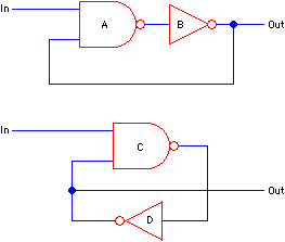
The raster method of node extraction views a layout as a unit grid of points, each of which is completely filled with zero or more layers [Baker and Terman]. Such a view is called a raster image since it changes the layout into a form that can be scanned in a regular and rectangular manner. Analysis is done in this raster scan order by passing a window over the image and examining the window's contents (see Fig. 5.1). As the window is moved, the lower-right corner is always positioned over a new element of the design. This element is assigned a node number based on the contents and node numbers of the other elements in the window. In fact, since this method is valid only for Manhattan geometry, the window need be only 2 × 2 because there are only two other elements of importance in this window: the element above and the element to the left of the new point.
 |
| FIGURE 5.1 Raster-based circuit analysis: (a) First position of window (b) Second position of window (c) Raster order. |
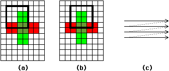
| Rules for assigning node numbers are very simple (see Fig. 5.2). If the new point in the lower-right corner is not connected to its adjoining points, it is given a new node number because it is on the upper-left corner of a new net. If the new point connects to one of its neighbors, then it is a downward or rightward continuation of that net and is given the same node number. If both neighbors connect to the new point and have the same node number, then this is again a continuation of a path. However, if the new point connects to both neighbors, and they have different node numbers, then this point is connecting two nets. It must be assigned a new node number and all three nets must be combined. Node-number combination is accomplished by having a table of equivalences in which each entry contains a true node number. The table must be as large as the maximum number of different net pieces that will be encountered, which can be much larger than the actual number of nets in the layout. Special care must be taken to ensure that transistor configurations and other special layer combinations are handled correctly in terms of net change and connectivity. |
|
When the entire layout has been scanned, an array of node numbers is available that can be used to tell which two points are connected. It is necessary to walk recursively through this table when determining true node numbers since a net may be equivalenced multiple times. Nevertheless, this information is easily converted to a netlist that shows components and their connections.
Network connectivity can also be determined from the adjacency and overlap of polygons that compose a design. Although many algorithms exist for this polygon evaluation, it helps to transform the polygons before analysis. In one system, all polygons are converted to strips that abut along only horizontal lines. This enables node extraction to proceed sequentially down the layout with simple comparison methods [McCormick].
Active components such as MOS transistors must be handled specially since they may contain single polygons that describe multiple nodes. The diffusion layer polygon must be split at the center of the transistor so that each half can be given a different node number.
In general, it is difficult to recognize all the special combinations of polygons that form different components. A common approach is to use libraries of component shapes to detect strange configurations without undue computation [McCormick; Chiba, Takashima, and Mitsuhashi; Takashima, Mitsuhashi, Chiba, and Yoshida]. This works because CAD systems often use regular and predictable combinations of polygons when creating complex components.
Once a network has been derived from a completed layout, it is useful to know whether this is the desired network. Although simulation and other network analyses can tell much about circuit correctness, only the designer knows the true topology, and would benefit from knowing whether the derived network is the same.
Often, an IC designer will first enter a circuit as a schematic and then produce the layout geometry to correspond. Since these operations are both done manually, the comparison of the original schematic with the node-extracted layout is informative. The original schematic network has known and correct topology, but the network derived from the IC layout is less certain. The goal is to compare these networks by associating the individual components and connections. If all of the parts associate, the networks are the same; if there are unassociated parts, these indicate how the networks differ.
Unfortunately, the comparison of two networks is a potentially impossible task when the networks are large. If the components of one network can be selected in order and given definite associations with the corresponding components in the other network, the entire comparison process is very fast. However, if uncertain choices are made and then rechosen during comparison as other dependent choices fail, this backtracking can take an unlimited amount of time to complete.
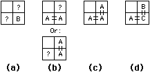
Many solutions to the problem make severe restrictions on the networks in order to function effectively. These restrictions attempt to reduce or eliminate the backtracking that occurs when an association between components is uncertain and must be tried and rejected. One set of restrictions organizes the networks in such a manner that they can both be traversed in a guaranteed path that must associate if the networks are equivalent [Baird and Cho]. The two restrictions that achieve this organization are a limit on the fan-out or fan-in, and a forced correspondence in the order of pin assignment on each component. The first restriction requires that every net have exactly one component that produces output to it. This associates components and nets with a one-to-one mapping, which makes network traversal easy. The use of wired-and or wired-or is disallowed and must be implemented with explicit components. Because every net is guaranteed to have exactly one source, it is possible to traverse the network, starting from the outputs, and reach every component in order.
| In Fig. 5.3, the two output pins correspond and are each driven by exactly one component (inverters B and D). With these inverters associated, it is next necessary to examine their inputs and determine the sources. In this example, each inverter has one input that is driven by the NAND gates A and C. Finally, the inputs of the NAND gates must be associated: One is from the inverter and the other is from the network input source. Note that this fan-in restriction of one output per net could be a fan-out restriction of one input per net if the algorithm worked instead from the inputs. All that matters is that every net have exactly one component that can be associated. |
|
The other necessary restriction to linearize search through a network is that the component's input connections are always assigned in the same order. Thus, for the previous example, each NAND gate's top input connection must be on the In signal and the bottom connection must feed back to the inverter. If one of the NAND gates has reversed inputs, then the traversal algorithm will fail. This restriction allows the nets to be associated correctly with no guesswork. However, it is a severe restriction that cannot always be guaranteed. One way of achieving this ordering is to "canonicalize" the input connections so that they are always ordered according to some network characteristic such as fan-out, wire length, or alphabetized net names. This may not work in all cases, so users must be allowed to correct the connection ordering if the network comparison has trouble. Of course, not all components have interchangeable inputs; so in most cases they will be properly ordered by design.
This network comparison scheme works well much of the time, but does have its shortcomings. For instance, certain pathological situations with strange connectivity may occur that cause the algorithm to loop. This can be overcome by marking components and nets as they are associated so that looping is detected. Also, bidirectional components such as MOS transistors could present a problem. Nevertheless, the comparison of networks is a necessary task that, even in its most restricted form, is useful in design.
When the restrictions on the networks described here are impossible to meet, other comparison schemes that take only slightly more time can be used. The method of graph isomorphism has been used successfully for network comparison [Ebeling and Zajicek; Spickelmier and Newton]. What graph isomorphism does is to classify every component according to as many characteristics as possible. Classifications include the component type, its connectivity (number of inputs and outputs), the type of its neighbors, and so on. After classification, the two networks are examined to find those classes that have only one component in each. These components are associated and the remaining components are reclassified. The purpose of reclassification is to take advantage of the information about previously associated components. Thus a new classification category is "number of neighbors already associated" and this information helps to aggragate additional associations about the initially distinct components.
Actual implementation of the graph-isomorphism process uses a hashing function to combine the component attributes into a single integer. This integer value is easier to tabulate. In addition, classification values from neighboring components can be combined into a component to refine its uniqueness further. The graph isomorphism technique of network comparison consumes time that is almost linear with the network size and is therefore competitive with the previously described method that restricts the network. Also, like the previous method, it is mostly unable to help identify problems when two networks differ.
|
Previous |  |
Table of Contents | Next | |
Static Free Software |  |