GNU Octave - Three-Dimensional Plotting

GNU Octave Manual Version 3
by John W. Eaton, David Bateman, Søren Hauberg
Paperback (6"x9"), 568 pages
ISBN 095461206X
RRP £24.95 ($39.95)

Get a printed copy>>>

GNU Octave Manual Version 3

Buy the book here >>>
support free documentation

15.1.2 Three-Dimensional Plotting

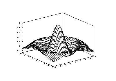
The function mesh produces mesh surface plots. For example,

tx = ty = linspace (-8, 8, 41)';
[xx, yy] = meshgrid (tx, ty);
r = sqrt (xx .^ 2 + yy .^ 2) + eps;
tz = sin (r) ./ r;
mesh (tx, ty, tz);

produces the familiar “sombrero” plot shown in Figure 15-5. Note the use of the function meshgrid to create matrices of X and Y coordinates to use for plotting the Z data. The ndgrid function is similar to meshgrid, but works for N-dimensional matrices.

Figure 15-5: Mesh plot.

The meshc function is similar to mesh, but also produces a plot of contours for the surface.

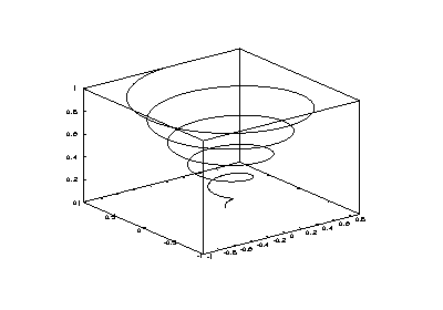
The plot3 function displays arbitrary three-dimensional data, without requiring it to form a surface. For example

t = 0:0.1:10*pi;
r = linspace (0, 1, numel (t));
z = linspace (0, 1, numel (t));
plot3 (r.*sin(t), r.*cos(t), z);

displays the spiral in three dimensions shown in Figure 15-6.

Figure 15-6: Three dimensional spiral.

Finally, the view function changes the viewpoint for three-dimensional plots.

Function File: mesh (x, y, z): Plot a mesh given matrices x, and y from meshgrid and a matrix z corresponding to the x and y coordinates of the mesh. If x and y are vectors, then a typical vertex is (x(j), y(i), z(i,j)). Thus, columns of z correspond to different x values and rows of z correspond to different y values.
See also meshgrid, contour

Function File: meshc (x, y, z): Plot a mesh and contour given matrices x, and y from meshgrid and a matrix z corresponding to the x and y coordinates of the mesh. If x and y are vectors, then a typical vertex is (x(j), y(i), z(i,j)). Thus, columns of z correspond to different x values and rows of z correspond to different y values.
See also meshgrid, mesh, contour

Function File: hidden (mode)
Function File: hidden (): Manipulation the mesh hidden line removal. Called with no argument the hidden line removal is toggled. The argument mode can be either 'on' or 'off' and the set of the hidden line removal is set accordingly.
See also mesh, meshc, surf

Function File: surf (x, y, z): Plot a surface given matrices x, and y from meshgrid and a matrix z corresponding to the x and y coordinates of the mesh. If x and y are vectors, then a typical vertex is (x(j), y(i), z(i,j)). Thus, columns of z correspond to different x values and rows of z correspond to different y values.
See also mesh, surface

Function File: surfc (x, y, z): Plot a surface and contour given matrices x, and y from meshgrid and a matrix z corresponding to the x and y coordinates of the mesh. If x and y are vectors, then a typical vertex is (x(j), y(i), z(i,j)). Thus, columns of z correspond to different x values and rows of z correspond to different y values.
See also meshgrid, surf, contour

Function File: [xx, yy, zz] = meshgrid (x, y, z)
Function File: [xx, yy] = meshgrid (x, y)
Function File: [xx, yy] = meshgrid (x): Given vectors of x and y and z coordinates, and returning 3 arguments, return three dimensional arrays corresponding to the x, y, and z coordinates of a mesh. When returning only 2 arguments, return matrices corresponding to the x and y coordinates of a mesh. The rows of xx are copies of x, and the columns of yy are copies of y. If y is omitted, then it is assumed to be the same as x, and z is assumed the same as y.
See also mesh, contour

Function File: [y1, y2, ..., yn] = ndgrid (x1, x2, ..., xn)

Function File: [y1, y2, ..., yn] = ndgrid (x)

Given n vectors x1, ... xn, ndgrid returns n arrays of dimension n. The elements of the i-th output argument contains the elements of the vector xi repeated over all dimensions different from the i-th dimension. Calling ndgrid with only one input argument x is equivalent of calling ndgrid with all n input arguments equal to x:

[y1, y2, ..., yn] = ndgrid (x, ..., x)

See also meshgrid

Function File: plot3 (args)

Produce three-dimensional plots. Many different combinations of arguments are possible. The simplest form is

plot3 (x, y, z)

in which the arguments are taken to be the vertices of the points to be plotted in three dimensions. If all arguments are vectors of the same length, then a single continuous line is drawn. If all arguments are matrices, then each column of the matrices is treated as a separate line. No attempt is made to transpose the arguments to make the number of rows match.

If only two arguments are given, as

plot3 (x, c)

the real and imaginary parts of the second argument are used as the y and z coordinates, respectively.

If only one argument is given, as

plot3 (c)

the real and imaginary parts of the argument are used as the y and z values, and they are plotted versus their index.

Arguments may also be given in groups of three as

plot3 (x1, y1, z1, x2, y2, z2, ...)

in which each set of three arguments is treated as a separate line or set of lines in three dimensions.

To plot multiple one- or two-argument groups, separate each group with an empty format string, as

plot3 (x1, c1, "", c2, "", ...)

An example of the use of plot3 is

   z = [0:0.05:5];
   plot3 (cos(2*pi*z), sin(2*pi*z), z, ";helix;");
   plot3 (z, exp(2i*pi*z), ";complex sinusoid;");