Diagonalizing a State-Space Model

To obtain the modal representation, we may diagonalize any state-space representation. This is accomplished by means of a particular similarity transformation specified by the eigenvectors of the state transition matrix $A$. An eigenvector of the square matrix $A$ is any vector $\underline{e}_i$ for which

$$A\underline{e}_i= \lambda_i \underline{e}_i,$$

where $\lambda_i$ may be complex. In other words, when the matrix $E$ of the similarity transformation is composed of the eigenvectors of $A$,

$$E= \left[ \underline{e}_1 \; \cdots \; \underline{e}_N \right],$$

the transformed system will be diagonalized, as we will see below.

A system can be diagonalized whenever the eigenvectors of $A$ are linearly independent. This always holds when the system poles are distinct. It may or may not hold when poles are repeated.

To see how this works, suppose we are able to find $N$ linearly independent eigenvectors of $A$, denoted $\underline{e}_i$, $i=1,\ldots,N$. Then we can form an $N\times N$ matrix $E$ having these eigenvectors as columns. Since the eigenvectors are linearly independent, $E$ is full rank and can be used as a one-to-one linear transformation, or change-of-coordinates matrix. From Eq. (E.19), we have that the transformed state transition matrix is given by

$$\tilde{A}= E^{-1}A E$$

Since each column $\underline{e}_i$ of $E$ is an eigenvector of $A$, we have $A\underline{e}_i=\lambda_i \underline{e}_i$, $i=1,\ldots,N$, which implies

$$A E= E\Lambda,$$

where

$$\Lambda \isdef \left[\begin{array}{ccc} \lambda_1 & & 0\\ [2pt] & \ddots & \\ [2pt] 0 & & \lambda_N \end{array}\right]$$

is a diagonal matrix having the (complex) eigenvalues of $A$ along the diagonal. It then follows that

$$\tilde{A}= E^{-1}A E= E^{-1}E\Lambda = \Lambda,$$

which shows that the new state transition matrix is diagonal and made up of the eigenvalues of $A$.

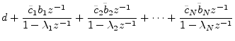
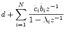
The transfer function is now, from Eq. (E.5), in the SISO case,

$$H(z) = d + {\tilde C}\left(zI - \Lambda\right)^{-1}{\tilde B}$$

$$= d + \frac{{\tilde c}_1 b_1 z^{-1}}{1 - \lambda _1z^{-1}} + \frac{... ...^{-1}} + \cdots + \frac{{\tilde c}_N {\tilde b}_N z^{-1}}{1 - \lambda _Nz^{-1}}$$

$$= d + \sum_{i=1}^N \frac{{\tilde c}_i {\tilde b}_i z^{-1}}{1 - \lambda _iz^{-1}} \protect$$ (E.22)

We have incidentally shown that the eigenvalues of the state-transition matrix $A$ are the poles of the system transfer function. When it is diagonal, i.e., when $A =$   diag$(\lambda _1,\ldots,\lambda _N)$, the state-space model may be called a modal representation of the system, because the poles appear explicitly along the diagonal of $A$ and the system's dynamic modes are decoupled.

Notice that the diagonalized state-space form is essentially equivalent to a partial-fraction expansion form (§6.8). In particular, the residue of the $i$th pole is given by $c_i b_i$. When complex-conjugate poles are combined to form real, second-order blocks (in which case $A$ is block-diagonal with $2\times 2$ blocks along the diagonal), this is corresponds to a partial-fraction expansion into real, second-order, parallel filter sections.