 |
(9.1) |
This chapter discusses pole-zero analysis of digital filters. Every digital filter can be specified by its poles and zeros (plus a gain factor). Poles and zeros give useful insights into a filter's response, and can be used as the basis for digital filter design. The Durbin step-down recursion for checking filter stability by finding the reflection coefficients is presented, including matlab code.
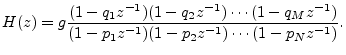
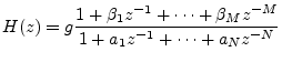
Going back to Eq. (6.5), we can write the general transfer function for the recursive LTI digital filter as
The term ``pole'' really makes sense when you plot the magnitude of
![]() as a function of z. Since
as a function of z. Since ![]() is complex, it may be taken to
lie in a plane (the
is complex, it may be taken to
lie in a plane (the ![]() plane). The magnitude of
plane). The magnitude of ![]() is real and
therefore can be represented by distance above the
is real and
therefore can be represented by distance above the ![]() plane. The plot
appears as an infinitely thin surface spanning in all directions over
the
plane. The plot
appears as an infinitely thin surface spanning in all directions over
the ![]() plane. The zeros are the points where the surface dips down to
touch the
plane. The zeros are the points where the surface dips down to
touch the ![]() plane. At high altitude, the poles look like thin, well,
``poles'' that go straight up forever, getting thinner the higher they
go.
plane. At high altitude, the poles look like thin, well,
``poles'' that go straight up forever, getting thinner the higher they
go.
Notice that the ![]() feedforward coefficients from the general
difference quation, Eq. (5.1), give rise to
feedforward coefficients from the general
difference quation, Eq. (5.1), give rise to ![]() zeros. Similarly,
the
zeros. Similarly,
the ![]() feedback coeficients in Eq. (5.1) give rise to
feedback coeficients in Eq. (5.1) give rise to ![]() poles. This illustrates the general fact that zeros are caused by
adding a finite number of input samples together and poles are caused
by feedback. Recall that the filter order is the maximum of
poles. This illustrates the general fact that zeros are caused by
adding a finite number of input samples together and poles are caused
by feedback. Recall that the filter order is the maximum of ![]() and
and
![]() . If
. If ![]() in Eq. (6.5), it then follows that the
filter order equals the number of poles or zeros, whichever is greater.
in Eq. (6.5), it then follows that the
filter order equals the number of poles or zeros, whichever is greater.
Recall that the order of a polynomial is defined as the highest
power of the polynomial variable. For example, the order of the
polynomial
![]() is 2. From Eq. (8.1), we see that
is 2. From Eq. (8.1), we see that ![]() is
the order of the transfer-function numerator polynomial in
is
the order of the transfer-function numerator polynomial in ![]() .
Similarly,
.
Similarly, ![]() is the order of the denominator polynomial in
is the order of the denominator polynomial in ![]() .
Therefore, the filter order is given by the maximum of the
numerator and denominator polynomial orders.
.
Therefore, the filter order is given by the maximum of the
numerator and denominator polynomial orders.