Sine-Wave Analysis

Suppose we test the filter at each frequency separately. This is called sine-wave analysis.^2.1Fig.1.6 shows an example of an input-output pair, for the filter of Eq. (1.1), at the frequency $f=f_s/4$ Hz, where $f_s$ denotes the sampling rate. (The continuous-time waveform has been drawn through the samples for clarity.) Figure 1.6a shows the input signal, and Fig.1.6b shows the output signal.

Figure 1.6: Input and output signals for the filter $y(n) = x(n) + x(n - 1)$. (a) Input sinusoid $x(n) = A_1 \sin(2\pi f n T + \phi_1)$ at amplitude $A_1=1$, frequency $f=f_s/4$, and phase $\phi _1=0$. (b) Output sinusoid $y(n) = A_2 \sin(2\pi f nT + \phi_2)$ at amplitude $A_2=1.414$, frequency $f=f_s/4$, and phase $\phi _2 = - \pi /4$.

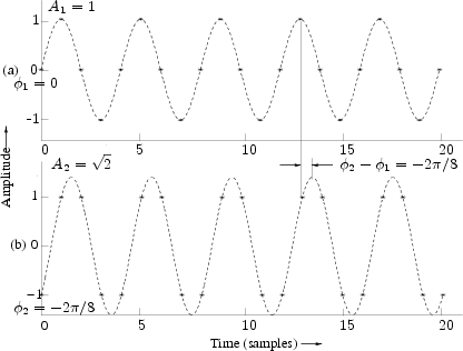The ratio of the peak output amplitude to the peak input amplitude is the filter gain at this frequency. From Fig.1.6 we find that the gain is about 1.414 at the frequency $f_s/4$. We may also say the amplitude response is 1.414 at $f_s/4$.

The phase of the output signal minus the phase of the input signal is the phase response of the filter at this frequency. Figure 1.6 shows that the filter of Eq. (1.1) has a phase response equal to $-2\pi/8$ (minus one-eighth of a cycle) at the frequency $f=f_s/4$.

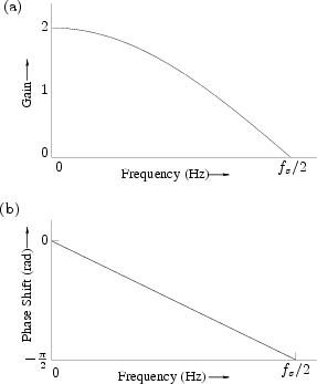
Continuing in this way, we can input a sinusoid at each frequency (from 0 to $f_s/2$ Hz), examine the input and output waveforms as in Fig.1.6, and record on a graph the peak-amplitude ratio (gain) and phase shift for each frequency. The resultant pair of plots, shown in Fig.1.7, is called the frequency response. Note that Fig.1.6 specifies the middle point of each graph in Fig.1.7.

Not every black box has a frequency response, however. What good is a pair of graphs such as shown in Fig.1.7 if, for all input sinusoids, the output is 60 Hz hum? What if the output is not even a sinusoid? We will learn in Chapter 4 that the sine-wave analysis procedure for measuring frequency response is meaningful only if the filter is linear and time-invariant (LTI). Linearity means that the output due to a sum of input signals equals the sum of outputs due to each signal alone. Time-invariance means that the filter does not change over time. We will elaborate on these technical terms and their implications later. For now, just remember that LTI filters are guaranteed to produce a sinusoid in response to a sinusoid--and at the same frequency.

Figure 1.7: Frequency response for the filter $y(n) = x(n) + x(n - 1)$. (a) Amplitude response. (b) Phase response.