State-Space Analysis Example:
The Digital Waveguide Oscillator

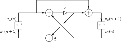
As an example of state-space analysis, we will use it to determine the frequency of oscillation of the system of Fig.E.3 [90].

Figure E.3: The second-order digital waveguide oscillator.

Note the assignments of unit-delay outputs to state variables $x_1(n)$ and $x_2(n)$. From the diagram, we see that

$$x_1(n+1) = c[x_1(n) + x_2(n)] - x_2(n) = c\,x_1(n) + (c-1) x_2(n)$$

and

$$x_2(n+1) = x_1(n) + c[x_1(n) + x_2(n)] = (1+c) x_1(n) + c\,x_2(n)$$

In matrix form, the state time-update can be written

$$\left[\begin{array}{c} x_1(n+1) \\ [2pt] x_2(n+1) \end{array}\rig... ...ay}\right]}_A \left[\begin{array}{c} x_1(n) \\ [2pt] x_2(n) \end{array}\right]$$

or, in vector notation,

$${\underline{x}}(n+1) = A \, {\underline{x}}(n).$$

We have two natural choices of output, $x_1(n)$ and $x_2(n)$:

$$\begin{eqnarray*} y_1(n) &\isdef & x_1(n) = [1, 0] {\underline{x}}(n)\\ y_2(n) &\isdef & x_2(n) = [0, 1] {\underline{x}}(n) \end{eqnarray*}$$

A basic fact from linear algebra is that the determinant of a matrix is equal to the product of its eigenvalues. As a quick check, we find that the determinant of $A$ is

$$\det{A} = c^2 - (c+1)(c-1) = c^2 - (c^2-1) = 1.$$

Since an undriven sinusoidal oscillator must not lose energy, and since every lossless state-space system has unit-modulus eigenvalues (consider the modal representation), we expect $\left\vert\det{A}\right\vert=1$.

Note that ${\underline{x}}(n) = A^n{\underline{x}}(0)$. If we diagonalize this system to obtain $\tilde{A}=E^{-1}A E$, where $\tilde{A}=$   diag$[\lambda_1,\lambda_2]$, and $E$ is the matrix of eigenvectors of $A$, then we have

$$\underline{{\tilde x}}(n) = \tilde{A}^n\,\underline{{\tilde x}}(0... ...t[\begin{array}{c} {\tilde x}_1(0) \\ [2pt] {\tilde x}_2(0) \end{array}\right]$$

where $\underline{{\tilde x}}(n) \isdef E^{-1}{\underline{x}}(n)$ denotes the state vector in these new ``modal coordinates''. Since $\tilde{A}$ is diagonal, the modes are decoupled, and we can write

$$\begin{eqnarray*} {\tilde x}_1(n) &=& \lambda_1^n\,{\tilde x}_1(0)\\ {\tilde x}_2(n) &=& \lambda_2^n\,{\tilde x}_2(0). \end{eqnarray*}$$

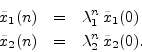
If this system is to generate a real sampled sinusoid at radian frequency $\omega$, the eigenvalues $\lambda_1$ and $\lambda_2$ must be of the form

$$\begin{eqnarray*} \lambda_1 &=& e^{j\omega T}\\ \lambda_2 &=& e^{-j\omega T}, \end{eqnarray*}$$

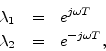
(in either order) where $\omega$ is real, and $T$ denotes the sampling interval in seconds.

Thus, we can determine the frequency of oscillation $\omega$ (and verify that the system actually oscillates) by determining the eigenvalues $\lambda_i$ of $A$. Note that, as a prerequisite, it will also be necessary to find two linearly independent eigenvectors of $A$ (columns of $E$).