


3.6 COVERAGEIn deployment applications one may be less interested in the expected value of some quantity, say travel time, than in the fraction of the city which receives "adequate coverage" by the service. Coverage is usually defined in terms of an inequality, such as travel time being less than or equal to 4.0 minutes. (For instance, The Emergency Medical Services Act of 1973 stipulates that 95 percent of ambulance responses should occur in Less than 30 minutes.7)In geometrical probability, coverage problems are defined in
terms of calculating the probabilities that certain
fixed geometrical figures or sets in the plane are covered by
other figures whose position is in some way random.
Several of these ideas extend directly to urban service systems,
as illustrated by example. 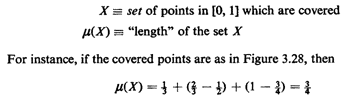
The points in X are usually determined according to some probabilistic process, and we wish to compute the expected value of u(X), Efu(X)]. 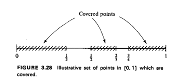
For example, suppose that we have N ambulettes distributed independently and uniformly over the interval [ - 'a, 1 + ja], the extensions beyond [0, 1] being added to avoid boundary problems. Emergency incidents are distributed uniformly on (0, 1] and are independent of ambulette positions. We want to know the expected amount of the interval [0, 1 ] which is "covered" by ambulettes, where a point is said to be covered if at least one ambulette is within a distance a/2 of the point.
Solution 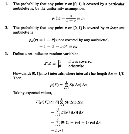
Hence, 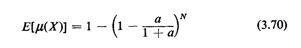
The approximate summation above becomes an integral when I 
 , ,
 x
0. Note that the solution behaves as we expect,
namely diminishing marginal returns (in terms of extra expected
area covered) with each additional ambulette. x
0. Note that the solution behaves as we expect,
namely diminishing marginal returns (in terms of extra expected
area covered) with each additional ambulette.
Generalizing the foregoing argument, if p(x) is the probability
that point x is covered,
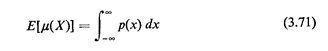
The generalization of this result from one dimension to n is known as "Robbins's theorem on random sets" (1944, 1945), and is discussed in Kendall and Moran [KEND 63, pp. 109-110]. We can extend (3.71) to obtain higher moments of
In practice, this formula is usually difficult to evaluate, even for second moments (m = 2). Thus, in our examples and assigned problems, we shall not concern ourselves with the higher moments.
Exercise 3.7: Including Boundary Effects Suppose in Example 10
that the ambulettes (as well as incidents) are
distributed uniformly and independently over [0, 1]. Show that
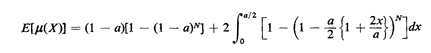
Question: How would you extend these coverage ideas to cases in which Nis a random variable? [This type of situation is likely to arise, for instance, in spatially distributed queueing systems (Chapter 5), in which a random number of units can be busy at any given time.] Exercise 3.8: N as a Random Variable Suppose that N is a
geometrically distributed random variable with mean E[N] =
1/q (0 < q < 1). For the original version of the one-dimensional
coverage problem (i.e., no boundary effects), show that
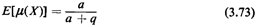
Does this result make sense for limiting values of a and q? Further work: Problem 3.23. Example 11: Coverage by Fixed-Position Ambulettes Ideas of coverage can also be applied to cases in which the response units (points on a line or on a grid) are fixed rather than random. As an example, imagine that ambulettes are prepositioned a unit distance apart at x = 0, � 1, � 2, . . . . Suppose that an emergency incident occurs and has random position. We wish to know the expected number of ambulettes within a distance t/2 of the incident (t > 0). This might be of interest for multiperson accidents requiring dispatch of two or more ambulettes. Solution
To solve this problem, instead of taking a random interval and a
fixed-integer
lattice, we can take a fixed interval and a lattice in random
position (reflecting
the point of view of the individuals at the incident's location).
Let the fixed
interval be t] and define a function
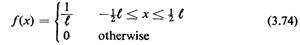
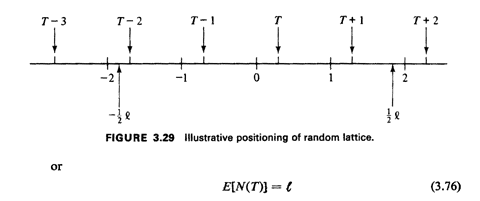
Note that f(x) is "like,, a pdf in Cat it is nonnegative and it integrates to 1; moreover, tf(x) is a "switching function," either "on" (equal to 1) or "off" (equal to 0). Let the lattice consist of the points T, T � 1, T � 2, . . . ,
where T is a random variable uniformly distributed over the
interval [0, 1]. Then the number of lattice points N(T) contained
in [-1/2 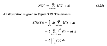
as we might have expected intuitively. This is a result that generalizes readily to two and more dimensions (see [KEND 63, pp. 102-104]). If t = p + q, where p is integral and 0 < q < 1, the variance is 
How did we obtain this result? Hint: Recognize (3.77) as the variance of a Bernoulli random variable. Question: Can you compare the mean coverage of the random position model (Example 10) to the mean coverage of the lattice-position model (Example 11) ? Further work: Problem 3.24. The coverage examples discussed above are illustrative of the types of problems that can be tackled using coverage concepts. However, apparently simple variations in coverage model assumptions seem to yield an intractable model much more readily than do models employing more conventional (non-area-based) random variables. 7 Federal law PL 93-154. Also see T. R. Willernain and R. C. Larson, eds., Emergency Medical Systems Analysis, Lexington Books, Lexington, Mass., 1977, especially pp. xxi-xxviii and 1-7. |
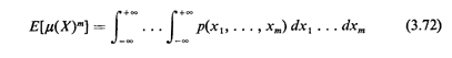
 (X). Suppose
p(x1, . . . , xm) is the probability that
x1,...,xm
all belong to the covered set X. Then
(X). Suppose
p(x1, . . . , xm) is the probability that
x1,...,xm
all belong to the covered set X. Then
 ,
,