First-Order Parallel Sections

Figure 3.9 shows the impulse response of the real one-pole section

$$H_1(z) = \frac{0.1657}{1 + 0.9z^{-1}},$$

and Fig.3.10 shows its frequency response, computed using the matlab utility myfreqz listed in §7.5.1. (Both Matlab and Octave have compatible utilities freqz, which serve the same purpose.) Note that the sampling rate is set to 1, and the frequency axis goes from 0 Hz all the way to the sampling rate, which is appropriate for complex filters (as we will soon see). Since real filters have Hermitian frequency responses (i.e., an even amplitude response and odd phase response), they may be plotted from 0 Hz to half the sampling rate without loss of information.

Figure 3.9: Impulse response of section 1 of the example filter.

Figure 3.10: Frequency response of section 1 of the example filter.

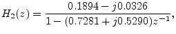
Figure 3.11 shows the impulse response of the complex one-pole section

$$H_2(z) = \frac{0.1894 - j 0.0326}{1 - (0.7281 + j 0.5290)z^{-1}},$$

and Fig.3.12 shows the corresponding frequency response.

Figure 3.11: Impulse response of complex one-pole section 2 of the full partial-fraction-expansion of the example filter.

Figure 3.12: Frequency response of complex one-pole section 2.

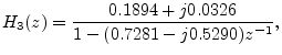
The complex-conjugate section,

$$H_3(z) = \frac{0.1894 + j 0.0326}{1 - (0.7281 - j 0.5290)z^{-1}},$$

is of course quite similar, and is shown in Figures 3.13 and 3.14.

Figure 3.13: Impulse response of complex one-pole section 3 of the full partial-fraction-expansion of the example filter.

Figure 3.14: Frequency response of complex one-pole section 3.

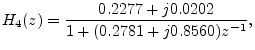
Figure 3.15 shows the impulse response of the complex one-pole section

$$H_4(z) = \frac{0.2277 + j 0.0202}{1 + (0.2781 + j 0.8560)z^{-1}},$$

and Fig.3.16 shows its frequency response. Its complex-conjugate counterpart, $H_5(z)$, is not shown since it is analogous to $H_4(z)$ in relation to $H_3(z)$.

Figure 3.15: Impulse response of complex one-pole section 4 of the full partial-fraction-expansion of the example filter.

Figure 3.16: Frequency response of complex one-pole section 4.